Tutorial: Add additional effects to simulated photometric fluxes#
By default, Phitter’s model binaries are located at a distance of 10 parsecs and simulated fluxes have no extinction applied. This means the output magnitudes are effectively apparent magnitudes. Phitter includes additional functions to modulate the simulated fluxes to account for distance modulus in magnitudes and reddening from extinction, which are covered in this tutorial. Additional functions exist in Phitter to modulate the simulated fluxes (see phitter.calc.phot_adj_calc), and are not covered in this tutorial.
Imports#
from phitter import observables, filters
from phitter.params import star_params, binary_params, isoc_interp_params
from phitter.calc import model_obs_calc, phot_adj_calc

import numpy as np

from phoebe import u
from phoebe import c as const
import matplotlib as mpl
import matplotlib.pyplot as plt

%matplotlib inline

# The following warning regarding extinction originates from SPISEA and can be ignored.
# The functionality being warned about is not used by SPISEA.
/Users/abhimat/Software/miniforge3/envs/phoebe_py38/lib/python3.8/site-packages/pysynphot/locations.py:345: UserWarning: Extinction files not found in /Volumes/Noh/models/cdbs/extinction
  warnings.warn('Extinction files not found in %s' % (extdir, ))
Set up model binary#
Let’s use the same red giant binary system we simulated in the previous tutorial.
filter_153m = filters.hst_f153m_filt()
filter_127m = filters.hst_f127m_filt()
# Object for interpolating stellar parameters from an isochrone

isoc_stellar_params_obj = isoc_interp_params.isoc_mist_stellar_params(
    age=8e9,
    met=0.0,
    use_atm_func='merged',
    phase='RGB',
    ext_Ks=2.2,
    dist=8e3*u.pc,
    filts_list=[filter_153m, filter_127m],
    ext_law='NL18',
)
star1_params = isoc_stellar_params_obj.interp_star_params_rad(
    15,
)

print("Star 1 Parameters")
print(star1_params)

star2_params = isoc_stellar_params_obj.interp_star_params_rad(
    12,
)

print("Star 2 Parameters")
print(star2_params)
Star 1 Parameters
mass_init = 1.103 solMass
mass = 1.100 solMass
rad = 15.000 solRad
lum = 70.325 solLum
teff = 4315.7 K
logg = 2.127
syncpar = 1.000
---
filt <phitter.filters.hst_f153m_filt object at 0x1087934c0>:
mag = 17.457
mag_abs = -1.909
pblum = 0.975 solLum
filt <phitter.filters.hst_f127m_filt object at 0x108793430>:
mag = 20.483
mag_abs = -1.431
pblum = 1.181 solLum

Star 2 Parameters
mass_init = 1.102 solMass
mass = 1.100 solMass
rad = 12.000 solRad
lum = 49.434 solLum
teff = 4418.1 K
logg = 2.321
syncpar = 1.000
---
filt <phitter.filters.hst_f153m_filt object at 0x1087934c0>:
mag = 17.883
mag_abs = -1.483
pblum = 0.659 solLum
filt <phitter.filters.hst_f127m_filt object at 0x108793430>:
mag = 20.887
mag_abs = -1.028
pblum = 0.815 solLum
# Binary parameters
bin_params = binary_params.binary_params(
    period = 30.0 * u.d,
    ecc = 0.2,
    inc = 80.0 * u.deg,
    t0 = 53_800.0,
)
# Set up model times
# Model times are in MJD here
model_phases = np.linspace(0, 1, num=100)
model_times = model_phases * bin_params.period.value + bin_params.t0
# Set up filter and observation type arrays for the model fluxes and RVs

flux_153m_filt_arr = np.full(len(model_phases), filter_153m)
flux_153m_type_arr = np.full(len(model_phases), 'phot')

flux_127m_filt_arr = np.full(len(model_phases), filter_127m)
flux_127m_type_arr = np.full(len(model_phases), 'phot')

rv_pri_filt_arr = np.full(len(model_phases), filter_153m)
rv_pri_type_arr = np.full(len(model_phases), 'rv_pri')

rv_sec_filt_arr = np.full(len(model_phases), filter_153m)
rv_sec_type_arr = np.full(len(model_phases), 'rv_sec')
# Now make arrays for all the times, filters, and observation types by concatenating the above arrays

obs_times = np.concatenate(
    (model_times, model_times, model_times, model_times),
)
obs_filts = np.concatenate(
    (flux_153m_filt_arr, flux_127m_filt_arr, rv_pri_filt_arr, rv_sec_filt_arr,),
)
obs_types = np.concatenate(
    (flux_153m_type_arr, flux_127m_type_arr, rv_pri_type_arr, rv_sec_type_arr,),
)
# Finally, construct the observables object

model_observables = observables.observables(
    obs_times=obs_times,
    obs_filts=obs_filts, obs_types=obs_types,
)
# Object to perform the computation of flux and RVs

binary_model_obj = model_obs_calc.binary_star_model_obs(
    model_observables,
    use_blackbody_atm=False,
    print_diagnostics=False,
)
modeled_observables = binary_model_obj.compute_obs(
    star1_params, star2_params, bin_params,
)
# Fluxes in mags
modeled_mags_153m = modeled_observables.obs[modeled_observables.phot_filt_filters[filter_153m]]

print(f'F153M-band mags: {modeled_mags_153m}')

modeled_mags_127m = modeled_observables.obs[modeled_observables.phot_filt_filters[filter_127m]]

print(f'F127M-band mags: {modeled_mags_127m}')

# RVs in km/s
modeled_rvs_star1 = modeled_observables.obs[modeled_observables.obs_rv_pri_filter]
modeled_rvs_star2 = modeled_observables.obs[modeled_observables.obs_rv_sec_filter]

print(f'Star 1 RVs: {modeled_rvs_star1} km/s')
print(f'Star 2 RVs: {modeled_rvs_star2} km/s')
F153M-band mags: [-2.07376567 -2.08993976 -2.07376567 -2.0991852  -2.15546044 -2.22491996
 -2.29432003 -2.35605566 -2.40597907 -2.44065194 -2.45367517 -2.45532707
 -2.45694645 -2.45838347 -2.45975778 -2.46113128 -2.46246321 -2.46355262
 -2.46466413 -2.46551129 -2.46661306 -2.46746037 -2.46813665 -2.46887976
 -2.46934813 -2.46992754 -2.47032046 -2.47075715 -2.47111439 -2.47116211
 -2.47125951 -2.47146599 -2.47156202 -2.47144126 -2.47138685 -2.47122224
 -2.4710011  -2.47067124 -2.47037411 -2.46992726 -2.46946711 -2.46882896
 -2.46829054 -2.46757638 -2.46683257 -2.46607895 -2.46515359 -2.46414984
 -2.46315754 -2.46204834 -2.46092315 -2.45969034 -2.45854065 -2.45706278
 -2.45585042 -2.45425752 -2.45295641 -2.43933153 -2.40171927 -2.34732274
 -2.28018805 -2.20541217 -2.13148578 -2.07237965 -2.04551215 -2.06079345
 -2.11251267 -2.1830001  -2.25757472 -2.32613203 -2.38318912 -2.42531764
 -2.44893931 -2.45376083 -2.45831062 -2.46348046 -2.46939025 -2.47568068
 -2.48202544 -2.48831559 -2.49376575 -2.49793381 -2.50065025 -2.50143559
 -2.50034338 -2.49730215 -2.49264282 -2.48698856 -2.480567   -2.47378547
 -2.46718838 -2.46100953 -2.45576449 -2.45046806 -2.42884237 -2.39063833
 -2.33887726 -2.27620657 -2.20714624 -2.14024233]
F127M-band mags: [-1.61029623 -1.62663852 -1.61029623 -1.6358076  -1.69236212 -1.76215011
 -1.83174369 -1.89339615 -1.94295009 -1.97704608 -1.98969145 -1.991178
 -1.99262742 -1.99389067 -1.995116   -1.9963313  -1.99752277 -1.9984585
 -1.99943488 -2.00015402 -2.00112902 -2.00186989 -2.00244946 -2.00309186
 -2.00346717 -2.00397875 -2.00429888 -2.00467477 -2.00495985 -2.00496719
 -2.00502061 -2.00518325 -2.00526509 -2.00513824 -2.00506564 -2.00490904
 -2.00468997 -2.00437908 -2.00410685 -2.00369562 -2.00327324 -2.00268483
 -2.00220894 -2.00155544 -2.00088769 -2.00022402 -1.99938824 -1.99848681
 -1.9976092  -1.9966183  -1.99562672 -1.9945315  -1.99353002 -1.99219404
 -1.99114931 -1.98971947 -1.9885937  -1.97502378 -1.93688921 -1.88109288
 -1.81178367 -1.73429714 -1.65765666 -1.59648019 -1.56870949 -1.58448922
 -1.63805517 -1.71128967 -1.78887502 -1.86011626 -1.91920457 -1.9625175
 -1.9865371  -1.99139327 -1.99594195 -2.00110355 -2.0069787  -2.01325522
 -2.01956889 -2.02586643 -2.03135186 -2.03557172 -2.03838394 -2.03929201
 -2.03833485 -2.03543336 -2.03091259 -2.02538485 -2.01905831 -2.01233145
 -2.00576286 -1.99957858 -1.9942999  -1.9889204  -1.96743857 -1.92933243
 -1.87744592 -1.81440613 -1.74479348 -1.67735338]
Star 1 RVs: [  8.96024086   2.97751958  -1.39149639  -4.21128267  -6.09344816
  -7.5183564   -8.8026365  -10.18734265 -12.04716593 -14.17764211
 -16.18991268 -18.09975825 -19.89607594 -21.58312924 -23.17086209
 -24.65291747 -26.0322593  -27.31479824 -28.49566213 -29.58421983
 -30.57638853 -31.48088871 -32.29518447 -33.0157848  -33.65197489
 -34.20112844 -34.66339391 -35.04120352 -35.3371882  -35.54753077
 -35.67686475 -35.72245268 -35.68198257 -35.56143318 -35.35962008
 -35.07093973 -34.69899518 -34.24248534 -33.69986432 -33.06749555
 -32.35266198 -31.54534657 -30.64944889 -29.6586031  -28.57184277
 -27.39574907 -26.11709733 -24.73822599 -23.2579385  -21.67107733
 -19.98379735 -18.18802279 -16.27909515 -14.26118298 -12.12920207
  -9.88891019  -7.52917459  -5.05870009  -2.47672279   0.21543058
   3.0094463    5.90776867   8.89393551  11.96827608  15.11012602
  18.31058181  21.546962    24.80048393  28.04178532  31.24491701
  34.37740099  37.3977694   40.26679173  42.94130402  45.38398488
  47.54845591  49.39806855  50.90399364  52.04906128  52.81064614
  53.18160126  53.16197407  52.75450554  51.96699174  50.80770409
  49.29845861  47.45617257  45.31163347  42.89543312  40.24094938
  37.39531831  34.41645618  31.90529969  29.74010527  27.72571683
  25.6573344   23.22869333  19.92575285  15.1431524    8.96024086] km/s
Star 2 RVs: [ -8.95730242  -5.97482556  -3.08288617  -0.2911698    2.39978047
   4.97957723   7.45210215   9.80974942  12.0583038   14.19236517
  16.21592921  18.1279848   19.93144006  21.6244964   23.21596394
  24.70345701  26.08612369  27.37265643  28.55939528  29.65072143
  30.64559812  31.54753219  32.36080101  33.08216947  33.71641412
  34.26392634  34.72487233  35.09893597  35.39125574  35.59523685
  35.71834294  35.7586531   35.7137181   35.58581399  35.37533122
  35.07850611  34.70000296  34.23405824  33.68181207  33.0447911
  32.31875224  31.50433461  30.59606969  29.59791278  28.50495013
  27.31746457  26.03279422  24.64694678  23.16235509  21.57226084
  19.87879755  18.07803786  16.17169235  14.15472151  12.02468016
  10.24656637   9.09500849   8.0965509    6.96559123   5.34313697
   2.63092808  -2.01757293  -8.8063555  -15.89326698 -21.10352454
 -24.35624001 -26.53371829 -28.28584588 -29.98835273 -31.88380026
 -34.22173561 -37.19538834 -40.0688389  -42.76530832 -45.24034591
 -47.45406972 -49.37433155 -50.96284924 -52.18731059 -53.02825494
 -53.46522424 -53.48644931 -53.09644481 -52.29983376 -51.10968411
 -49.55318678 -47.65469077 -45.45009213 -42.98386752 -40.28472383
 -37.40464532 -34.38062868 -31.25383689 -28.05531361 -24.81956821
 -21.57576276 -18.34787864 -15.1584592  -12.02461219  -8.95730242] km/s
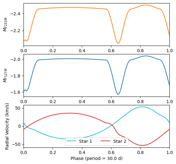
fig = plt.figure(figsize=(6,6))

# F153M mags subplot
ax_mag_153m = fig.add_subplot(3,1,1)

ax_mag_153m.plot(
    model_phases, modeled_mags_153m,
    '-', color='C1',
)

ax_mag_153m.set_xlim([0, 1])

ax_mag_153m.invert_yaxis()
ax_mag_153m.set_ylabel(r"$M_{F153M}$")

# F153M mags subplot
ax_mag_127m = fig.add_subplot(3,1,2)

ax_mag_127m.plot(
    model_phases, modeled_mags_127m,
    '-', color='C0',
)

ax_mag_127m.set_xlim([0, 1])

ax_mag_127m.invert_yaxis()
ax_mag_127m.set_ylabel(r"$M_{F127M}$")

# RVs subplot
ax_rvs = fig.add_subplot(3,1,3)

ax_rvs.plot(
    model_phases, modeled_rvs_star1,
    '-', color='C9', label='Star 1',
)

ax_rvs.plot(
    model_phases, modeled_rvs_star2,
    '-', color='C3', label='Star 2',
)

ax_rvs.set_xlabel(f"Phase (period = {bin_params.period:.1f})")
ax_rvs.set_xlim([0, 1])

ax_rvs.set_ylabel("Radial Velocity (km/s)")

ax_rvs.legend(loc='lower center', ncol=2)
<matplotlib.legend.Legend at 0x1689fa310>
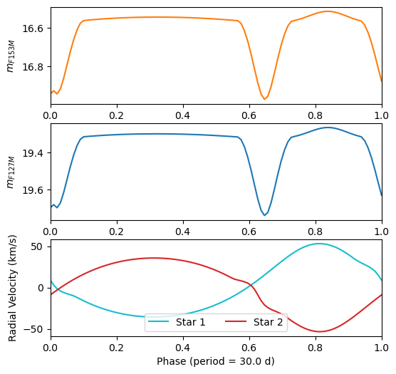
Add distance modulus#
Since our current binary’s mags are calculated for a distance of 10 parsecs, we need to add a distance modulus. Let’s put this star at the center of the Milky Way Galaxy, at a distance of 8 kpc.
modeled_observables = phot_adj_calc.apply_distance_modulus(
    modeled_observables,
    8e3*u.pc,
)
# Fluxes in mags
modeled_mags_153m = modeled_observables.obs[modeled_observables.phot_filt_filters[filter_153m]]
modeled_mags_127m = modeled_observables.obs[modeled_observables.phot_filt_filters[filter_127m]]

# RVs in km/s
modeled_rvs_star1 = modeled_observables.obs[modeled_observables.obs_rv_pri_filter]
modeled_rvs_star2 = modeled_observables.obs[modeled_observables.obs_rv_sec_filter]

# Draw plot
fig = plt.figure(figsize=(6,6))

# F153M mags subplot
ax_mag_153m = fig.add_subplot(3,1,1)

ax_mag_153m.plot(
    model_phases, modeled_mags_153m,
    '-', color='C1',
)

ax_mag_153m.set_xlim([0, 1])

ax_mag_153m.invert_yaxis()
ax_mag_153m.set_ylabel(r"$m_{F153M}$")

# F153M mags subplot
ax_mag_127m = fig.add_subplot(3,1,2)

ax_mag_127m.plot(
    model_phases, modeled_mags_127m,
    '-', color='C0',
)

ax_mag_127m.set_xlim([0, 1])

ax_mag_127m.invert_yaxis()
ax_mag_127m.set_ylabel(r"$m_{F127M}$")

# RVs subplot
ax_rvs = fig.add_subplot(3,1,3)

ax_rvs.plot(
    model_phases, modeled_rvs_star1,
    '-', color='C9', label='Star 1',
)

ax_rvs.plot(
    model_phases, modeled_rvs_star2,
    '-', color='C3', label='Star 2',
)

ax_rvs.set_xlabel(f"Phase (period = {bin_params.period:.1f})")
ax_rvs.set_xlim([0, 1])

ax_rvs.set_ylabel("Radial Velocity (km/s)")

ax_rvs.legend(loc='lower center', ncol=2)
<matplotlib.legend.Legend at 0x168cc9b80>
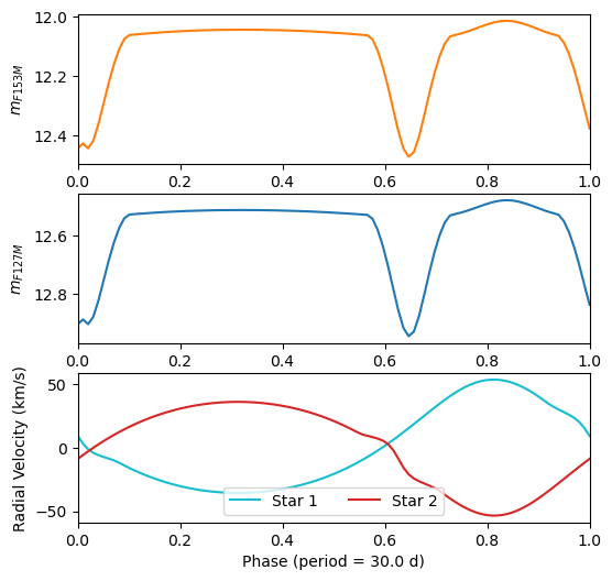
Apply reddening from extinction#
Extinction in Phitter is applied using a power-law extinction law, typically specified in the form $A_{\lambda} \propto \lambda^{-\alpha}$, where $A_{\lambda}$ is the extinction at wavelength $\lambda$ and $\alpha$ is the power-law slope
In order to modulate the extinction from the synthetic photometryu calculated during the creation of the isochrone, we need to provide the following inputs:
bin_observables = modeled_observables: The input observables to be modeled.isoc_Ks_ext = 2.2: The Ks-band extinction that the initial isochrone was generated with.ref_filt = filter_153m: The filter where we will provide the desired extinction. Extinction in other bands will be computed based on this extinction and the provided extinction power-law slope ($\alpha$ inext_alpha).target_ref_filt_ext = bin_ext: The extinction in the reference filter needs to be specified. Extinction in all other passbands will be modulated in reference to this value.ext_alpha = bin_ext_alpha: The extinction power-law slope ($\alpha$).isoc_red_law = 'NL18': The extinction law that was used when computing the synthetic photometry during isochrone generation.
modeled_observables = phot_adj_calc.apply_extinction(
    modeled_observables,
    isoc_Ks_ext=2.2,
    ref_filt=filter_153m,
    target_ref_filt_ext=4.5,
    isoc_red_law='NL18',
    ext_alpha=2.23,
)
# Fluxes in mags
modeled_mags_153m = modeled_observables.obs[modeled_observables.phot_filt_filters[filter_153m]]
modeled_mags_127m = modeled_observables.obs[modeled_observables.phot_filt_filters[filter_127m]]

# RVs in km/s
modeled_rvs_star1 = modeled_observables.obs[modeled_observables.obs_rv_pri_filter]
modeled_rvs_star2 = modeled_observables.obs[modeled_observables.obs_rv_sec_filter]

# Draw plot
fig = plt.figure(figsize=(6,6))

# F153M mags subplot
ax_mag_153m = fig.add_subplot(3,1,1)

ax_mag_153m.plot(
    model_phases, modeled_mags_153m,
    '-', color='C1',
)

ax_mag_153m.set_xlim([0, 1])

ax_mag_153m.invert_yaxis()
ax_mag_153m.set_ylabel(r"$m_{F153M}$")

# F153M mags subplot
ax_mag_127m = fig.add_subplot(3,1,2)

ax_mag_127m.plot(
    model_phases, modeled_mags_127m,
    '-', color='C0',
)

ax_mag_127m.set_xlim([0, 1])

ax_mag_127m.invert_yaxis()
ax_mag_127m.set_ylabel(r"$m_{F127M}$")

# RVs subplot
ax_rvs = fig.add_subplot(3,1,3)

ax_rvs.plot(
    model_phases, modeled_rvs_star1,
    '-', color='C9', label='Star 1',
)

ax_rvs.plot(
    model_phases, modeled_rvs_star2,
    '-', color='C3', label='Star 2',
)

ax_rvs.set_xlabel(f"Phase (period = {bin_params.period:.1f})")
ax_rvs.set_xlim([0, 1])

ax_rvs.set_ylabel("Radial Velocity (km/s)")

ax_rvs.legend(loc='lower center', ncol=2)
<matplotlib.legend.Legend at 0x168e88c70>