Tutorial: Simulate a model binary#
This tutorial walks through the basics of using phitter to compute light curves and RVs for a model stellar binary.
Imports#
from phitter import observables, filters
from phitter.params import star_params, binary_params, blackbody_params
from phitter.calc import model_obs_calc

import numpy as np

from phoebe import u
from phoebe import c as const
import matplotlib as mpl
import matplotlib.pyplot as plt

%matplotlib inline

# The following warning regarding extinction originates from SPISEA and can be ignored.
# The functionality being warned about is not used by SPISEA.
/Users/abhimat/Software/miniforge3/envs/phoebe_py38/lib/python3.8/site-packages/pysynphot/locations.py:345: UserWarning: Extinction files not found in /Volumes/Noh/models/cdbs/extinction
  warnings.warn('Extinction files not found in %s' % (extdir, ))
Set up observation filters / passbands#
For this example, we’re going to generate photometry and RVs in Keck Kp band. Any passband set up in both PHOEBE and SPISEA can be used by Phitter for simulating fluxes and RVs.
filter_kp = filters.nirc2_kp_filt()
Set up stellar and binary system parameters#
Stellar parameters#
We’re going to set up parameters for the component stars in the binary system with photometry derived from a blackbody. This requires providing mass, radius, and temperature for each star.
# Star parameters

bb_stellar_params_obj = blackbody_params.bb_stellar_params()

star1_params = bb_stellar_params_obj.calc_star_params(
    50 * u.solMass, 52 * u.solRad, 30_000 * u.K,
)

star2_params = bb_stellar_params_obj.calc_star_params(
    45 * u.solMass, 45 * u.solRad, 25_000 * u.K,
)
Set up a binary parameters object#
A separate object is set up to specify the parameters of the binary system
# Binary parameters
bin_params = binary_params.binary_params(
    period = 20.0 * u.d,
    ecc = 0.05,
    inc = 80.0 * u.deg,
    t0 = 53_800.0,
)
Set up of observables to be calculated#
We need to set up an observables object to specify the times and types of observables that need to be computed. For this example, let’s compute flux in Keck K-band and RVs uniformly over the entire orbital phase of the binary.
# Set up model times
# Model times are in MJD here
model_phases = np.linspace(0, 1, num=100)
model_times = model_phases * bin_params.period.value + bin_params.t0
# Set up filter and observation type arrays for the model fluxes and RVs

kp_filt_arr = np.full(len(model_phases), filter_kp)
kp_type_arr = np.full(len(model_phases), 'phot')

rv_pri_filt_arr = np.full(len(model_phases), filter_kp)
rv_pri_type_arr = np.full(len(model_phases), 'rv_pri')

rv_sec_filt_arr = np.full(len(model_phases), filter_kp)
rv_sec_type_arr = np.full(len(model_phases), 'rv_sec')
# Now make arrays for all the times, filters, and observation types by concatenating the above arrays

obs_times = np.concatenate(
    (model_times, model_times, model_times),
)
obs_filts = np.concatenate(
    (kp_filt_arr, rv_pri_filt_arr, rv_sec_filt_arr,),
)
obs_types = np.concatenate(
    (kp_type_arr, rv_pri_type_arr, rv_sec_type_arr,),
)
# Finally, construct the observables object

model_observables = observables.observables(
    obs_times=obs_times,
    obs_filts=obs_filts, obs_types=obs_types,
)
Compute the observables#
First a model observation calculation object (model_obs_calc) has to be instantiated, with the observables as input parameters. This object will be carrying out the calculations.
# Object to perform the computation of flux and RVs

binary_model_obj = model_obs_calc.binary_star_model_obs(
    model_observables,
    use_blackbody_atm=True,
    print_diagnostics=False,
)
The modeled observables can then be simulated by inputting the stellar and binary parameters.
modeled_observables = binary_model_obj.compute_obs(
    star1_params, star2_params, bin_params,
)
Process and plot the modeled observables#
We can extract the different observables (flux and RVs of the primary and secondary object) from the output observables object. The observables object has numpy filters for each passband and data types that we can use for this.
# Fluxes in mags
modeled_kp_mags = modeled_observables.obs[modeled_observables.phot_filt_filters[filter_kp]]

print(f'Kp-band mags: {modeled_kp_mags}')

# RVs in km/s
modeled_rvs_star1 = modeled_observables.obs[modeled_observables.obs_rv_pri_filter]
modeled_rvs_star2 = modeled_observables.obs[modeled_observables.obs_rv_sec_filter]

print(f'Star 1 RVs: {modeled_rvs_star1} km/s')
print(f'Star 2 RVs: {modeled_rvs_star2} km/s')
Kp-band mags: [-7.5216657  -7.53732926 -7.5216657  -7.53973471 -7.58422804 -7.6434513
 -7.70671535 -7.76850532 -7.82567567 -7.87684326 -7.92123227 -7.9589559
 -7.98949251 -8.01222054 -8.02392512 -8.02926534 -8.03464135 -8.03978097
 -8.04512171 -8.05026785 -8.05499389 -8.05965313 -8.06381118 -8.06742234
 -8.0707711  -8.07336674 -8.0753406  -8.07691355 -8.07784988 -8.07791415
 -8.07786586 -8.07681172 -8.07544044 -8.07313791 -8.0702784  -8.06746169
 -8.0638797  -8.05981414 -8.05567433 -8.05147333 -8.04686716 -8.04234265
 -8.03770362 -8.03263123 -8.0182408  -7.99586114 -7.96713968 -7.93223797
 -7.89169488 -7.8463103  -7.79686441 -7.74500755 -7.69428287 -7.65015828
 -7.62135114 -7.61633102 -7.63662295 -7.6757046  -7.7243426  -7.77576576
 -7.82591875 -7.8724258  -7.91454599 -7.95108773 -7.98218025 -8.00744218
 -8.0265221  -8.0384456  -8.04556605 -8.05304594 -8.06062383 -8.06820929
 -8.0752654  -8.08167704 -8.08702932 -8.09139645 -8.09415882 -8.09548854
 -8.09522449 -8.09383937 -8.09062861 -8.08629899 -8.08040402 -8.0734608
 -8.0655998  -8.05723694 -8.04857565 -8.03984411 -8.03170232 -8.02326546
 -8.00664823 -7.98281403 -7.95231821 -7.91482576 -7.87066209 -7.81978953
 -7.76289086 -7.70152922 -7.63835483 -7.5803122 ]
Star 1 RVs: [   8.3645588   -20.72126128  -42.78321712  -57.33403586  -66.82057916
  -73.40743418  -78.48141781  -82.79790172  -86.81473427  -90.87297976
  -95.17329818  -99.99513811 -106.16950658 -113.14473386 -119.59989517
 -125.55295565 -130.9919105  -135.88108371 -140.29568743 -144.16538332
 -147.52139283 -150.36323497 -152.68049597 -154.49586261 -155.82593365
 -156.57922333 -156.8680753  -156.64458017 -155.90614339 -154.67592131
 -152.94370496 -150.70965628 -147.98012086 -144.7153373  -140.9567258
 -136.76601174 -132.00254521 -126.75365832 -121.01008446 -114.81700743
 -108.12273938 -100.99997401  -93.39910259  -85.3842781   -76.97976576
  -68.19792792  -59.04069552  -49.57086978  -39.81711275  -29.78706422
  -19.55885966   -9.12678602    1.43364637   12.08601054   22.81407832
   33.53972245   44.20659904   54.80346614   65.23094339   75.44727086
   85.41728951   95.06716457  104.33120411  113.18878257  121.53341727
  129.32082842  136.53697068  143.07943596  148.97988595  154.18420839
  158.71292283  162.53692469  165.69212759  168.21006382  170.04745492
  171.21145367  171.69995938  171.45932309  170.53705681  168.93993298
  166.63771821  163.6308055   159.89544385  155.42984771  150.22590561
  144.2864683   137.58360979  130.33004141  124.0580466   118.38509998
  113.12074107  108.10089376  103.18221374   98.07183948   92.31597699
   85.15214354   75.16779889   60.16406811   37.64145169    8.3645588 ] km/s
Star 2 RVs: [  -9.30041204    2.50410814   14.16562647   25.67206929   36.94494359
   47.97531301   58.69174249   69.12035131   79.16694275   88.81417575
   98.04413382  106.83285253  115.15213351  122.9893872   130.30413878
  137.10017692  143.35255178  149.07128874  154.20704145  158.79735648
  162.80580603  166.2663088   169.10218567  171.38539398  173.06966805
  174.16508265  174.6643893   174.57883199  173.89271835  172.63868982
  170.74759035  168.30877263  165.28297836  161.68059288  157.46400701
  152.71996893  147.38982022  141.50576497  135.06435162  128.10485559
  120.60515754  112.70100092  106.69837965  101.79244882   97.47733391
   93.4133502    89.33096789   84.87011687   79.39775618   71.8552754
   60.31299594   41.65245503   13.26456234  -21.70464555  -53.21215397
  -75.12448441  -88.92807004  -97.94153472 -104.53558441 -109.95958671
 -114.98414704 -119.97830835 -125.2164007  -130.86963335 -137.18480064
 -144.68052272 -152.87248756 -160.38885062 -167.16675609 -173.20117313
 -178.45298833 -182.88248841 -186.48124599 -189.23931305 -191.19961314
 -192.243635   -192.49423607 -191.85823293 -190.38154407 -188.05011772
 -184.87109601 -180.90651511 -176.11474404 -170.55151307 -164.21340472
 -157.14966866 -149.38135158 -140.9742126  -131.96817453 -122.39822833
 -112.33723958 -101.83936398  -90.97014566  -79.7680786   -68.32052664
  -56.69329864  -44.903312    -33.03154919  -21.13607745   -9.30041204] km/s
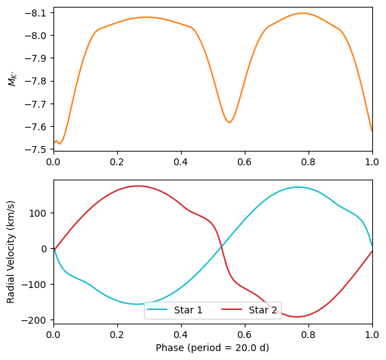
Now that we have the modeled observables, we can plot them for this model binary
fig = plt.figure(figsize=(6,6))

# Kp mags subplot
ax_mag_kp = fig.add_subplot(2,1,1)

ax_mag_kp.plot(
    model_phases, modeled_kp_mags,
    '-', color='C1',
)

ax_mag_kp.set_xlim([0, 1])

ax_mag_kp.invert_yaxis()
ax_mag_kp.set_ylabel(r"$M_{K'}$")

# RVs subplot
ax_rvs = fig.add_subplot(2,1,2)

ax_rvs.plot(
    model_phases, modeled_rvs_star1,
    '-', color='C9', label='Star 1',
)

ax_rvs.plot(
    model_phases, modeled_rvs_star2,
    '-', color='C3', label='Star 2',
)

ax_rvs.set_xlabel(f"Phase (period = {bin_params.period:.1f})")
ax_rvs.set_xlim([0, 1])

ax_rvs.set_ylabel("Radial Velocity (km/s)")

ax_rvs.legend(loc='lower center', ncol=2)
<matplotlib.legend.Legend at 0x16c180100>
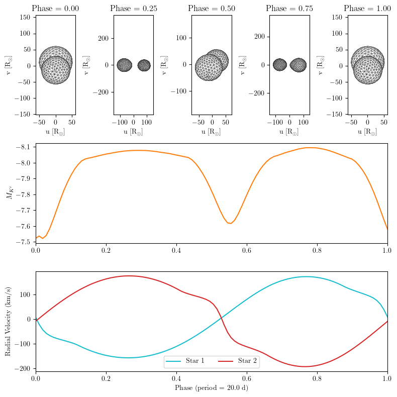
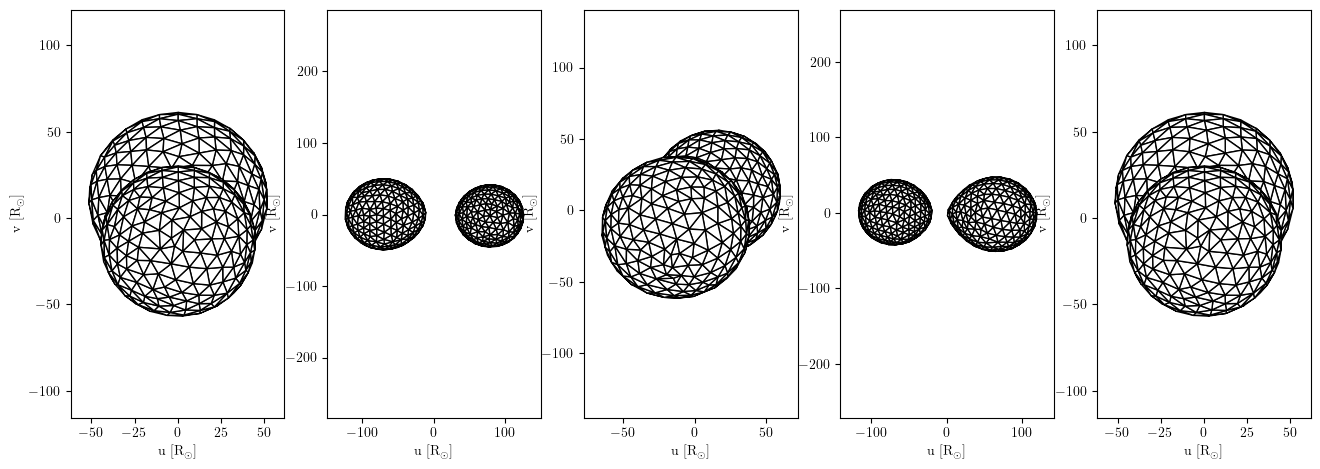
Bonus: make mesh plots to aide visualization#
The above plot is great to see the modeled observables. But it can be helpful to see what the modeled binary system looks like. Let’s add simulate some mesh outlines of the stellar surfaces to see what this model binary looks like…
We need to make a figure first where we’ll do the plotting. We can be extra specific about the layout of the mesh plots in this figure, so let’s do that!
# Set up figure and specificy mesh plot outputs

fig = plt.figure(figsize=(8,8))
gs = plt.GridSpec(5, 5,)

mesh_plot_phases = np.array([0.0, 0.25, 0.5, 0.75, 1.0])

modeled_observables, mesh_plot_out, fig = binary_model_obj.compute_obs(
    star1_params, star2_params, bin_params,
    make_mesh_plots=True,
    mesh_plot_phases=mesh_plot_phases,
    mesh_plot_fig=fig,
    mesh_plot_subplot_grid=(3,5),
    mesh_plot_subplot_grid_indexes=np.array([1, 2, 3, 4, 5,]),
    num_triangles=500,
)

# The mesh subplots show here since we have matplotlib inline enabled
# Finish constructing the whole figure

# Fluxes in mags
modeled_kp_mags = modeled_observables.obs[modeled_observables.phot_filt_filters[filter_kp]]

# RVs in km/s
modeled_rvs_star1 = modeled_observables.obs[modeled_observables.obs_rv_pri_filter]
modeled_rvs_star2 = modeled_observables.obs[modeled_observables.obs_rv_sec_filter]

# Label the mesh subplots
# # Remove empty axes
# for ax in fig.axes:
#     if ax.get_xlabel() == '':
#         ax.remove()

# # Make mesh axes share axes
# mesh_axes = []

for ax_index, phase in enumerate(mesh_plot_phases):
    ax = fig.axes[ax_index]

    ax.set_title(f'Phase = {phase:.2f}')

    # Decrease linewidths of the triangles in the mesh, for legibility in final plot
    for child in ax.get_children():
        if isinstance(child, mpl.collections.PolyCollection):
            child.set(lw=0.25)

    # mesh_axes.append(ax)

# Draw observables subplots
# Kp mags subplot
ax_mag_kp = fig.add_subplot(3,1,2)

ax_mag_kp.plot(
    model_phases, modeled_kp_mags,
    '-', color='C1',
)

ax_mag_kp.set_xlim([0, 1])

ax_mag_kp.invert_yaxis()
ax_mag_kp.set_ylabel(r"$M_{K'}$")

# RVs subplot
ax_rvs = fig.add_subplot(3,1,3)

ax_rvs.plot(
    model_phases, modeled_rvs_star1,
    '-', color='C9', label='Star 1',
)

ax_rvs.plot(
    model_phases, modeled_rvs_star2,
    '-', color='C3', label='Star 2',
)

ax_rvs.set_xlabel(f"Phase (period = {bin_params.period:.1f})")
ax_rvs.set_xlim([0, 1])

ax_rvs.set_ylabel("Radial Velocity (km/s)")

ax_rvs.legend(loc='lower center', ncol=2)

fig.set_size_inches(8, 8)
fig.tight_layout()

fig